Learning with Kernels

These are a set of study notes on the mathematics of kernels. They are largely based on Schölkopf and Smola’s *Learning with Kernels [1]. They study the theory of reproducing kernel Hilbert spaces, and kernelized algorithms for machine learning, and connect these to kernel integral operators and their regularization properties.*

1. Support Vector Machines

Let’s start at the very beginning, a very good place to start.

The simplest learning problem we can start with is classifying datapoints into two buckets. Here, we imagine our data lives in $\mathcal{X}$ (drawn as $\mathbb{R}^2$), and the ‘true’ categories live in $\mathcal{Y} = \{+1,-1\}$, drawn as blue and red dots respectively.

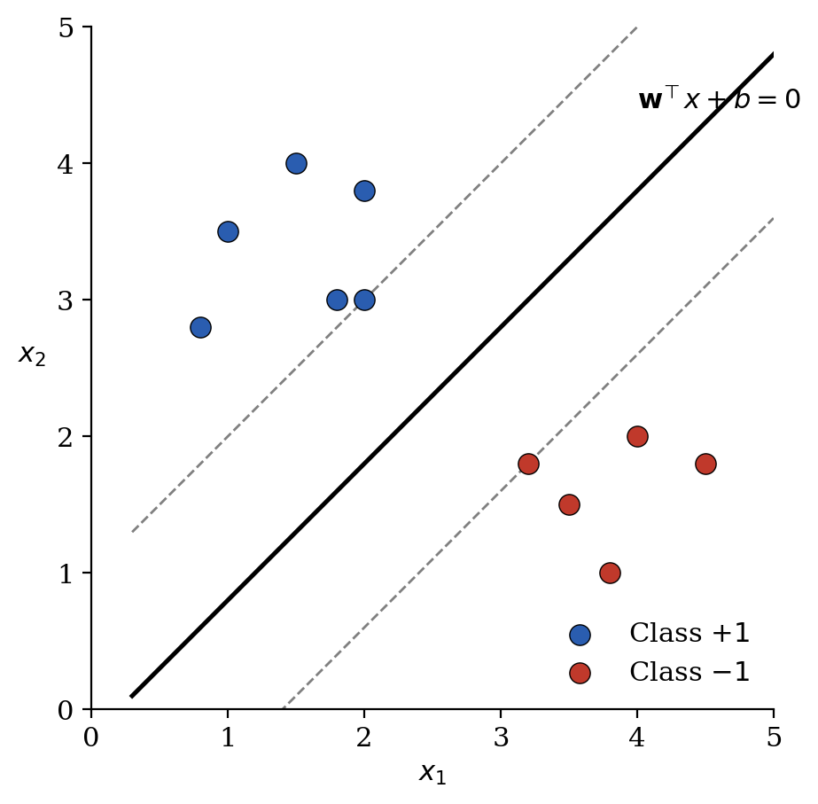
This problem is fairly easy to solve. A hyperplane is specified by

So we want to find a hyperplane $\mathbf{w}, b$ such that the distance between

is maximal. We set up the following optimization problem, and fit the optimal $\mathbf{w}, b$ using various techniques in convex optimization (we solve the dual problem using Lagrange multipliers):

This setup does not allow us to misclassify even a single data point: the hard constraints mean that if even a single data point is too noisy, the model will have no output. In practice we allow for some loosening according to a hyperparameter $\lambda$. The second term below is known as the hinge loss:

Choosing $\lambda = \infty$ recovers the hard-classification problem.

A much harder problem to solve, however, is the following.

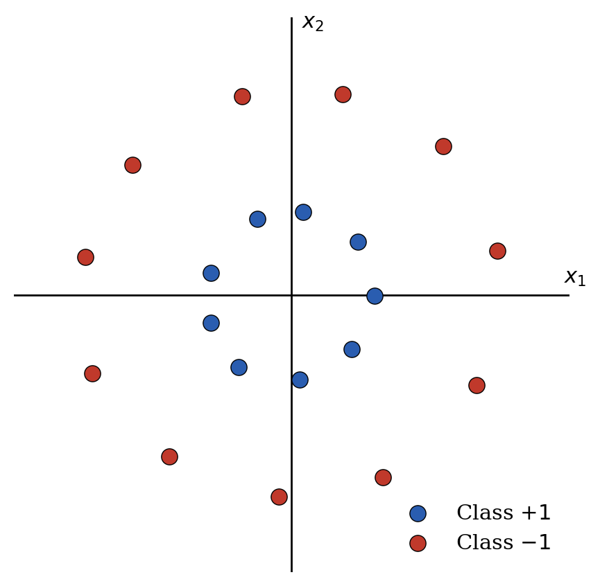
To our eyes, this problem is simple: we can quickly see that the classifying curve is a circle between the two classes. However, this is where the nonlinearity becomes a problem: our technique only allows us to learn a hyperplane.

The trick is to define a feature map $\varphi(x_1,x_2) = (x_1, x_2, x_1^2 + x_2^2)$, and lift to a higher-dimensional space, where the classification problem is completely linear.

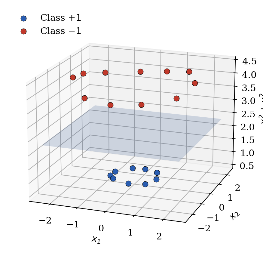
In this new picture, the data is again linearly separable, with the separating hyperplane now being $2$-dimensional instead of $1$-dimensional.

The issue, of course, is that in this example, we knew the ‘correct’ feature map. In practice, for data that is naturally much higher-dimensional and scattered, we can’t read off the ‘correct’ feature map just by looking at it.

Another option is to simply try a huge dictionary and let the model learn a large number of zero weights. For example, we could try a much more general feature map like

which has all polynomial terms of degree $2$. This approach is promising, and would indeed work on our second example: we would learn some hyperplane that depends on $x_1^2 + x_2^2$ and be done. Let us do some back-of-the-envelope math to see if this method generalizes. Assume our data comes from a $d$-dimensional space (in our toy example, $d = 2$), and as a heuristic for our feature space, we choose all monomials of degree at most $n$ (in the previous example, $n = 2$). The number of monomials is then

which grows very fast in $d$. The features soon become too vast to compute efficiently. Just throwing in more and more features runs into the curse of dimensionality very quickly.

What we would like is a method to pick small feature maps based on how important we think they will be, in a data-driven way. The kernel trick provides a way to systematically construct such feature maps, without ever explicitly choosing features by hand.

2. The Kernel Trick

The basic kernel trick is as follows: assume our data $\{x_i\}$ comes from a set $X$. We place no structure on $X$: it need not have any inner product or linear structure. We then define a kernel $k(x,y) : X \times X \to \mathbb{R}$. We require some mild assumptions on $k$, in particular that it be a positive-semidefinite function (which we shall define later). Under these assumptions, the kernel implicitly defines a feature map $\varphi : X \to \mathcal{H}$: there exists some Hilbert space $\mathcal{H}$ such that

This avoids the curse of dimensionality, since we never actually have to compute $\varphi$ explicitly: the choice of kernel lets us compute inner products in this space without it.

Designing good kernels is as much an art as a science, but the heuristic is that, since it behaves like a cosine similarity, the kernel should measure ‘similarity’ in a sense that is useful to us, and the associated feature map will then find a high-dimensional embedding that is useful to us.

The “kernel trick” means different things to different people. Here are a few benefits of working with kernels, all of which are often referred to as the ‘kernel trick’:

1. A choice of kernel lets us implicitly choose a dictionary of feature maps, rather than doing so explicitly, which might be better adapted to the problem at hand.
2. It solves the curse-of-dimensionality problem in picking a large dictionary.
3. It lets us lift a lower-dimensional problem to a higher-dimensional one.
4. It lets us put linear structure on problems that might not have any natural linear structure (string or image kernels).
5. Any algorithm that only accesses the data through inner products can be reinterpreted as a kernelized algorithm.

These notes work through each of these benefits in detail.

3. Reproducing Kernel Hilbert Spaces

The previous section begs the question: what is this magical high-dimensional $\mathcal{H}$ into which our kernel is embedding the data? The answer is that it is a reproducing kernel Hilbert space, which we define and prove some basic facts about below. For this section, we work with vector spaces over $\mathbb{R}$ for simplicity.

Definition 3.1. A reproducing kernel Hilbert space (RKHS) is a Hilbert space $H$ where point evaluation is continuous: for each $x$, the map $f \mapsto f(x)$ is bounded, i.e. $\lvert f(x)\rvert \leq M_x |f|_H$.

Then $f(x) = \langle f, K_x\rangle$ by the Riesz Representation Theorem, where $K_x(\cdot) = K(x, \cdot)$.

Not every Hilbert space is an RKHS. For example, $L^2([0,1])$ is not a reproducing kernel Hilbert space, since a function $f \in L^2([0,1])$ can be unbounded at any single point while remaining square-integrable.

We can define $k(x,y) = \langle K_y, K_x\rangle$ to be the kernel of this space. This function is symmetric and positive-definite, since inner products are symmetric and positive-definite in their arguments. The important fact is that the converse also holds.

Theorem 3.2 (Moore–Aronszajn). For any symmetric positive-definite kernel $k(x,y) : \mathcal{X} \times \mathcal{X} \to \mathbb{R}$, there exists a unique RKHS $H$ for which $k$ is the reproducing kernel.

Proof. We define a vector space $H_0$ as

with the inner product

This is a well-defined inner product, due to the symmetric, positive-definite nature of the kernel. We then define $H$ to be the closure of $H_0$ in the induced norm. We can interpret $H$ as the space of functions $f : \mathcal{X} \to \mathbb{R}$ of the form $f(x) = \sum_{i=1}^n \alpha_i k(x_i, x)$. Almost by construction, $H$ has the reproducing property.

To see uniqueness, suppose there is another Hilbert space $H’$ for which $k$ is the reproducing kernel. Define $\iota : H \to H’$ to be the linear map sending $K_x = K(x,\cdot) \in H_0$ to $K_x = K(x,\cdot) \in H’$. This is injective, and the inner product on $H’$ must agree with that on $H$ by linearity. Since $H’$ is complete, taking closures gives $H \subseteq H’$.

Now let $g \in H’$ with $g \perp H$, so that $\langle g, K_x \rangle_{H’} = 0$ for all $x \in X$. By the reproducing property of $H’$, $g(x) = 0$ for all $x$, i.e. $g$ is the zero function. Thus $\iota$ is an isometric isomorphism. $\square$

In this space, the feature map $\varphi : \mathcal{X} \to H$ is given by $x \mapsto k(x, \cdot)$. This is a complete, precise, and unique characterization of the Hilbert space, but it is not so useful for reasoning geometrically about the feature space. To do so, we add some more assumptions and give a second characterization.

4. Mercer’s Theorem

Now we assume more structure on our state space $X$: let $X$ be a compact metric space with a probability measure $\mu$, and let $L^2(X, \mu)$ denote the square-integrable functions.

Suppose $k(x,y) : X \times X \to \mathbb{R}$ is symmetric, and let its kernel integral operator be $T_k f(x) = \int_X k(x,y) f(y)\, d\mu(y)$. Then $T_k$ is self-adjoint, since for any $f, g$,

One can further show that $k$ being positive-semidefinite implies $T_k$ is a positive operator, i.e. $\langle T_k f, f\rangle \geq 0$ for all $f$. We claim $T_k$ is compact when $k$ is continuous.

Theorem 4.1. Let $k : X \times X \to \mathbb{R}$ be continuous. Then $T_k$ is compact.

Proof. Let $B = \{f \in L^2(\mu) : \lVert f\rVert = 1\}$ be the unit ball in $L^2(X, \mu)$. We show that $T_k(B)$ is pointwise bounded and equicontinuous, so that by Arzelà–Ascoli it is relatively compact in the uniform topology of $C(X)$. Since the inclusion $C(X) \hookrightarrow L^2(X,\mu)$ is continuous, this suffices.

For pointwise boundedness,

For equicontinuity, let $\varepsilon > 0$. Then

Since $k$ is continuous on a compact set, it is uniformly continuous, and hence so is $(x,y) \mapsto \int \lvert k(x,t) - k(y,t)\rvert\, d\mu(t)$. $\square$

Since $T_k$ is compact and self-adjoint, it has an orthonormal basis of eigenvectors $\psi_i$ with eigenvalues $\lambda_i$ satisfying $\lvert\lambda_i\rvert \to 0$. Since $T_k$ is positive, each $\lambda_i \geq 0$.

Theorem 4.2 (Mercer). For a symmetric positive-definite kernel $k(x,y) : X \times X \to \mathbb{R}$,

where the sum on the right converges absolutely, and if $k$ is continuous, uniformly.

Proof. Assume throughout that $\mu$ has full support; otherwise everything below holds with $\operatorname{supp}\mu$ in place of $X$. Write

and let $r_n(x) = k_n(x,x)$ be the diagonal defect.

Step 1: the eigenfunctions are continuous. If $\lambda_i > 0$ then $\psi_i = \lambda_i^{-1} T_k \psi_i$, so it is enough that $T_k$ maps $L^2(\mu)$ into $C(X)$. By Cauchy–Schwarz,

and $k$ is uniformly continuous on the compact space $X \times X$, so the right-hand side tends to $0$ as $x’ \to x$. Hence we may take every $\psi_i$ with $\lambda_i > 0$ continuous, and each $k_n$ is continuous.

Step 2: the diagonal bound. The integral operator of $k_n$ is $T_k$ precomposed with the orthogonal projection onto $\operatorname{span}\{\psi_1, \ldots, \psi_n\}^{\perp}$, so $T_{k_n} \geq 0$. A continuous kernel with a positive integral operator is nonnegative on the diagonal: if $k_n(x_0,x_0) < 0$ then by continuity $k_n < 0$ on $B \times B$ for some ball $B \ni x_0$, and testing against $\chi_B$ gives $\langle T_{k_n}\chi_B, \chi_B\rangle < 0$ — using $\mu(B) > 0$, which is where full support is needed. Therefore $r_n \geq 0$, i.e.

so $\sum_{i=1}^\infty \lambda_i \psi_i(x)^2$ converges at every $x$, with sum at most $k(x,x)$.

Step 3: absolute convergence. By Cauchy–Schwarz, for $m \leq n$,

By Step 2 the right-hand side tends to $0$ as $m \to \infty$, so $k_0(x,y) := \sum_{i=1}^\infty \lambda_i \psi_i(x)\psi_i(y)$ converges absolutely at every point, with $\lvert k_0\rvert \leq M$. Since each $k_n$ is a continuous kernel with $T_{k_n} \geq 0$, it obeys the Cauchy–Schwarz inequality for positive-semidefinite kernels, which controls the whole square by the diagonal:

Step 4: $k_0 = k$. Fix $x$. The function $k(x,\cdot)$ lies in $L^2(\mu)$ and its Fourier coefficients against the basis are $\langle k(x,\cdot), \psi_i\rangle = T_k\psi_i(x) = \lambda_i \psi_i(x)$. It is also orthogonal to $\ker T_k$, since $\psi \in \ker T_k$ gives $\langle k(x,\cdot), \psi\rangle = T_k\psi(x) = 0$. Hence $s_n(x,\cdot) \to k(x,\cdot)$ in $L^2(\mu)$. But by Step 3, $s_n(x,\cdot) \to k_0(x,\cdot)$ pointwise and boundedly, so also in $L^2(\mu)$. Therefore $k(x,y) = k_0(x,y)$ for $\mu$-almost every $y$, for every $x$.

Step 5: uniform convergence. It remains to see that $r_n \to 0$ pointwise, which upgrades Step 4 to equality everywhere. Since $r_n$ is a decreasing sequence of continuous nonnegative functions, $\int_X r_n\, d\mu = \int_X k(x,x)\, d\mu(x) - \sum_{i \leq n}\lambda_i$, so $r_n \downarrow 0$ pointwise exactly when

the trace identity for continuous positive-definite kernels. This is the substantive input to Mercer’s theorem, and we take it as known here. Granted it, $r_n$ is a decreasing sequence of continuous functions converging pointwise to the continuous function $0$ on a compact space, so by Dini’s theorem the convergence is uniform. Feeding this back into the bound of Step 3,

so the expansion converges uniformly, and absolutely by Step 3. $\square$

5. Risk Minimization

Definition 5.1. A loss function is a map $c : X \times Y \times Y \to [0, \infty)$ that takes an input $x$, an observation $y$, and a prediction $f(x)$ to a nonnegative real number, satisfying $c(x,y,y) = 0$.

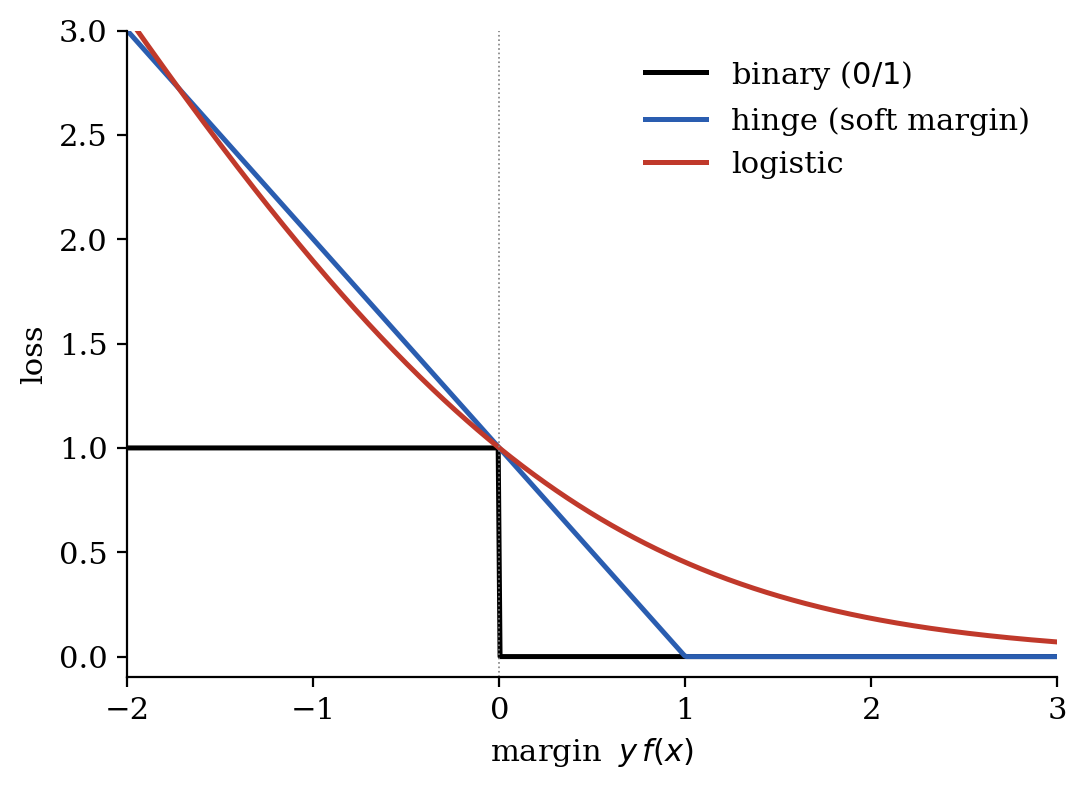
There are a number of common loss functions. The first three are used for classification, where $Y = \{-1, +1\}$, and it is natural to express the loss in terms of the margin $y f(x)$: a positive margin means $f$ predicts the correct sign, and a larger margin means a more confident correct prediction.

• Binary (0–1) loss. This simply counts misclassifications:

It is the loss we truly care about, but it is non-convex and discontinuous, so in practice we minimize a convex surrogate that upper-bounds it. The next two are the most common such surrogates.

• Soft margin (hinge) loss. Penalizes any point whose margin falls short of $1$:

This is the loss underlying the support vector machine of Section 1.

• Logistic loss. A smooth surrogate arising from logistic regression:

The remaining two are used for regression, where $Y = \mathbb{R}$, and depend on the residual $f(x) - y$.

• Squared (mean-square) loss. $c(x,y,f(x)) = (f(x)-y)^2$. Smooth and strongly convex, but sensitive to outliers.
• $L^1$ loss. $c(x,y,f(x)) = \lvert f(x)-y\rvert$. More robust to outliers, but not differentiable at $0$.

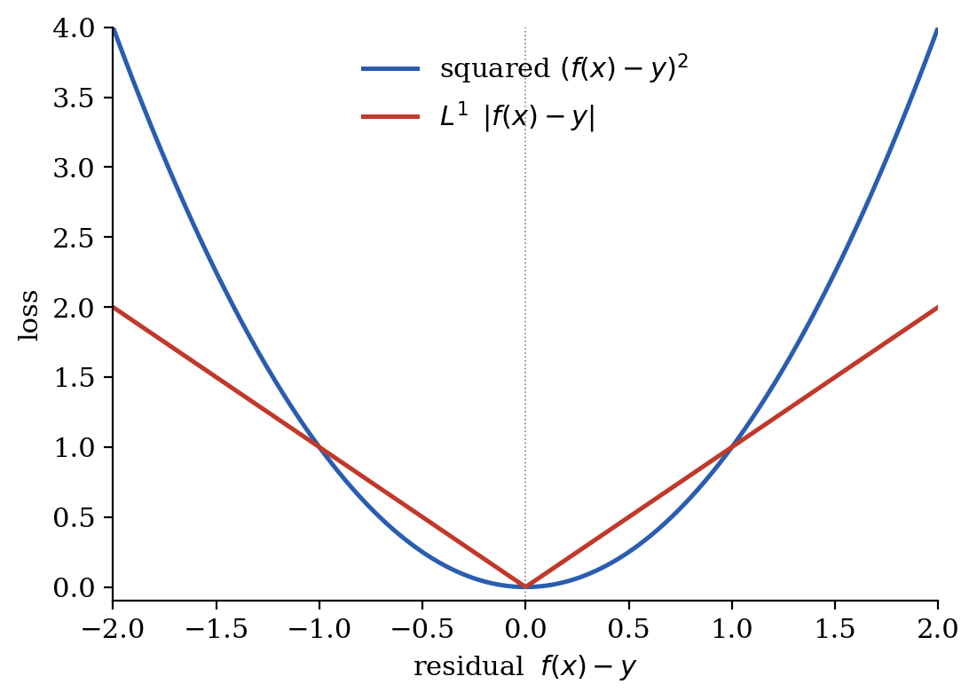
Each of these satisfies the axiom $c(x,y,y) = 0$: a perfect prediction incurs no loss.

In practice we assume our data comes from some probability distribution $P(x,y)$ on $X \times Y$, and we want to minimize the expected loss over this distribution to find a function $f_\ast$. We fix a function space $\mathcal{F}$ in which to optimize, and solve

Of course, in practice we do not have access to the full distribution $P(x,y)$. We instead have a training set of size $n$, which we write as

We are thus forced to minimize the empirical risk,

We call the function being minimized the empirical risk functional $R(f) = \frac{1}{n} \sum_{i=1}^n c(x_i,y_i,f(x_i))$.

In theory we want $\mathcal{F}$ as rich as possible. But this leads to problems. First, adding more functions to our optimization space can make the problem numerically ill-conditioned. Second, we risk overfitting: the empirical minimizer perfectly remembers the training data but performs badly out of sample. It is also possible that we have some prior (in the Bayesian sense) about what the solution should look like. In any case, it is often useful to add a regularization term of the form $\Omega(f)$, where $\Omega$ is some (generally convex) positive functional that builds in the properties we want. The problem we solve becomes

Here $\lambda$ is the regularization parameter: small $\lambda$ regularizes weakly, large $\lambda$ regularizes strongly. We now leave statistical learning theory aside and focus on the mathematical problem of actually solving this.

6. The Representer Theorem

Reproducing kernel Hilbert spaces are in general infinite-dimensional, and optimizing over an infinite-dimensional space sounds hard. However — and this is the heart of the kernel trick — the representer theorem tells us that it is tractable: the best fit to the data $\{x_i\}$ is a finite linear combination of the feature vectors $K(x_i, \cdot)$. We therefore only need to learn finitely many coefficients.

Theorem 6.1 (Representer Theorem). Given a training sample $(x_1, y_1), \ldots, (x_n, y_n) \in X \times \mathbb{R}$, a loss function $L : X \times \mathbb{R} \times \mathbb{R} \to \mathbb{R}$, and a strictly increasing $\Omega$, the minimizer in $H$ of

is of the form

Proof. Let

Since this is finite-dimensional it is closed, so the projection onto it and its orthogonal complement are well-defined. Write $f = f_\parallel + f_\perp$ with $f_\parallel \in H_n$ and $f_\perp \perp H_n$. Then

so the loss term depends only on $f_\parallel$:

But $\lVert f\rVert_H^2 = \lVert f_\parallel\rVert_H^2 + \lVert f_\perp\rVert_H^2 \geq \lVert f_\parallel\rVert_H^2$. Thus the first term of the risk depends only on $f_\parallel$, while the regularization term is only increased by a nonzero $f_\perp$. Hence $\lVert f_\perp\rVert = 0$ for the optimal $f$, which means $f \in \text{span}\{K(x_i, \cdot)\}_i$. $\square$

7. Kernel Mean Embedding

Until now, we have worked on lifting single data points into a reproducing kernel Hilbert space. We can work one level higher, and embed entire probability distributions into RKHSs. Here we assume $M$ is compact and the kernel $k$ is continuous. By $P(M)$ we denote the space of finite Borel measures on $M$. The kernel mean embedding induced by a kernel $k$ is the map $E : P(M) \to \mathcal{H}$ given by

We say that a kernel $k(x,y)$ is characteristic if the induced map $E$ is injective on probability distributions. In practice we assume a stronger property on our kernels: that they are in fact universal.

Definition 7.1. A kernel $k : M \times M \to \mathbb{R}$ is universal if the reproducing kernel Hilbert space $\mathcal{H}$ is dense in $C_b(M)$: for every $f \in C_b(M)$ and every $\varepsilon > 0$ there exists $h \in \mathcal{H}$ with $\lVert h - f\rVert_\infty < \varepsilon$.

This embedding induces a pseudometric on the space of probability measures: given $\mu_1, \mu_2$, set

This is known as the maximum mean discrepancy (MMD). To see its relationship to other metrics on the space of probability distributions, we define the notion of an integral probability metric.

Definition 7.2. Given two probability measures $\mu_1$ and $\mu_2$ on a measurable space $\mathcal{X}$, an integral probability metric (IPM) is

where $\mathcal{F}$ is a space of real-valued bounded measurable functions on $\mathcal{X}$.

The function class $\mathcal{F}$ fully characterizes the IPM $\gamma[\mathcal{F}, \mu_1, \mu_2]$, and there is an obvious trade-off in choosing it. On one hand, the class must be rich enough that $\gamma[\mathcal{F}, \mu_1, \mu_2]$ vanishes if and only if $\mu_1 = \mu_2$. On the other, the larger the class, the harder $\gamma[\mathcal{F}, \mu_1, \mu_2]$ is to estimate. For example, taking $\mathcal{F}$ to be all bounded continuous functions on $\mathcal{X}$ does give a metric on probability distributions.

Since $C_b(\mathcal{X})$ is difficult to work with in practice, we use more restrictive classes:

• Taking $\mathcal{F}{\mathrm{TV}} = \{ f : \lVert f\rVert\infty \leq 1 \}$, where $\lVert f\rVert_\infty = \sup_{\mathbf{x} \in \mathcal{X}} \lvert f(\mathbf{x})\rvert$, gives $\gamma[\mathcal{F}_{\mathrm{TV}}, \mu_1, \mu_2] = \lVert \mu_1 - \mu_2\rVert_1$, the total variation distance.
• Writing $\lVert f\rVert_L := \sup\{ \lvert f(\mathbf{x}) - f(\mathbf{y})\rvert / \rho(\mathbf{x}, \mathbf{y}) : \mathbf{x} \neq \mathbf{y} \in \mathcal{X} \}$ for the Lipschitz semi-norm with respect to a metric $\rho$ on $\mathcal{X}$, and taking $\mathcal{F}_{\mathrm{W}} = \{ f : \lVert f\rVert_L \leq 1 \}$, yields the Wasserstein $W_1$ distance (sometimes called the earthmover distance).

8. Random Fourier Features

In Section 6 we saw that optimizing over an infinite-dimensional RKHS $\mathcal{H}$ reduces to learning a finite number of coefficients $\{\alpha_i\}$, one per data point:

Mathematicians tend to be quite happy with reducing a possibly infinite-dimensional problem to a finite one. However, in modern machine learning datasets are enormous, and it is not practical to learn as many coefficients as you have data points. So instead of evaluating the kernel at every data point, we use a random approximation to $k(x_i, x)$ built from $D$ functions, indexed by $\omega_j$ and chosen independently of the data:

Since a linear combination of a linear combination is just another linear combination, we can write

reducing the problem to learning a relatively small number of coefficients. The question is how to build that approximation well. To do so, we restrict to translation-invariant kernels.

Definition 8.1. A translation-invariant kernel is a kernel $k(x,y)$ that depends only on $x - y$. With a slight abuse of notation, we write $k(x,y) = k(x-y)$.

Such kernels admit an abstract characterization via Bochner’s theorem.

Theorem 8.2 (Bochner). A (normalized) translation-invariant kernel $k(x-y)$ can be written as the Fourier transform of a finite Borel probability measure: there exists a measure $\Lambda(\omega)$ such that

This measure $\Lambda$ is called the spectral measure. It gives us a way to write randomized kernel algorithms: draw samples $\{\omega_j\}_{j=1}^D \sim d\Lambda$ and approximate the integral by a sum,

This relies on being able to compute and sample from the spectral measure. Luckily, most commonly used kernels have easily computed spectral measures. For example, the Gaussian kernel $k(x-y) = \exp!\left(-\lVert x-y\rVert^2 / 2\sigma^2\right)$ on $\mathbb{R}^K$ has spectral measure

which is just another Gaussian, and very easy to sample from.

We can further use Hoeffding’s inequality to bound the approximation error, which decays like $O(1/\sqrt{D})$ in the number $D$ of random features. In practice we can do much better than this bound and get away with far fewer features: ‘random features’ form a perfectly good (random) basis by themselves, and can be used directly. The interested reader is referred to [2].

It is also worth noting that this perspective can be used to understand neural networks rigorously. A neural network with a single hidden layer tends, in the infinite-width limit, to a kernel machine. That limit corresponds precisely to taking infinitely many random features, so a real-world finite-width single-layer network can be understood as a random Fourier features method. This is particularly interesting because ML theory lacks a rigorous understanding of real-world neural networks, and this is a useful toy model for them.

References

[1] B. Schölkopf and A. J. Smola, Learning with Kernels: Support Vector Machines, Regularization, Optimization, and Beyond, MIT Press, 2002.

[2] A. Rahimi and B. Recht, “Random Features for Large-Scale Kernel Machines,” Advances in Neural Information Processing Systems, 2007.