Notes on Ergodic Theory

These are a set of study notes on ergodic theory, with a special view toward studying dynamical systems via their Koopman operator.

They are largely structured around two textbooks: Operator-Theoretic Aspects of Ergodic Theory [1] and An Introduction to Ergodic Theory [2], as well as lectures given by Dimitris Giannakis at Dartmouth College in Spring 2025. They were written for the Mathematics Directed Reading Program (DRP) at Dartmouth in the Winter of 2026.

The general construction of a dynamical system is that there is some phase space $X$, with a dynamical map $T: X \to X$, and we study the properties of this map, and trajectories under it. There are two typical settings for this: we can either assume $X$ is a topological space, and the dynamics are continuous, or that $X$ is a measure space, and the dynamics are measurable. There is a deep and rich interplay between these two settings, but for now we will set everything up in the latter formalism.

1. Measure-Preserving Dynamical Systems

Definition 1.1. A dynamical system $(X, \mathcal{X}, \mu, T)$ consists of a measure space $(X, \mathcal{X}, \mu)$ (also known as the phase space) along with a measurable map $T: X \to X$ such that the measure is invariant under the dynamics. That is, for any measurable set $S \in \mathcal{X}$, we have $\mu(T^{-1}(S)) = \mu(S)$.

Note that for ease of notation, we will often omit the $\sigma$-algebra unless necessary, and assume subsets to be measurable.

We can often assume or show that the measure preserved by the dynamics is finite. Without loss of generality, we then normalize it such that it is a probability measure.

Let’s work out some examples.

Examples 1.2.

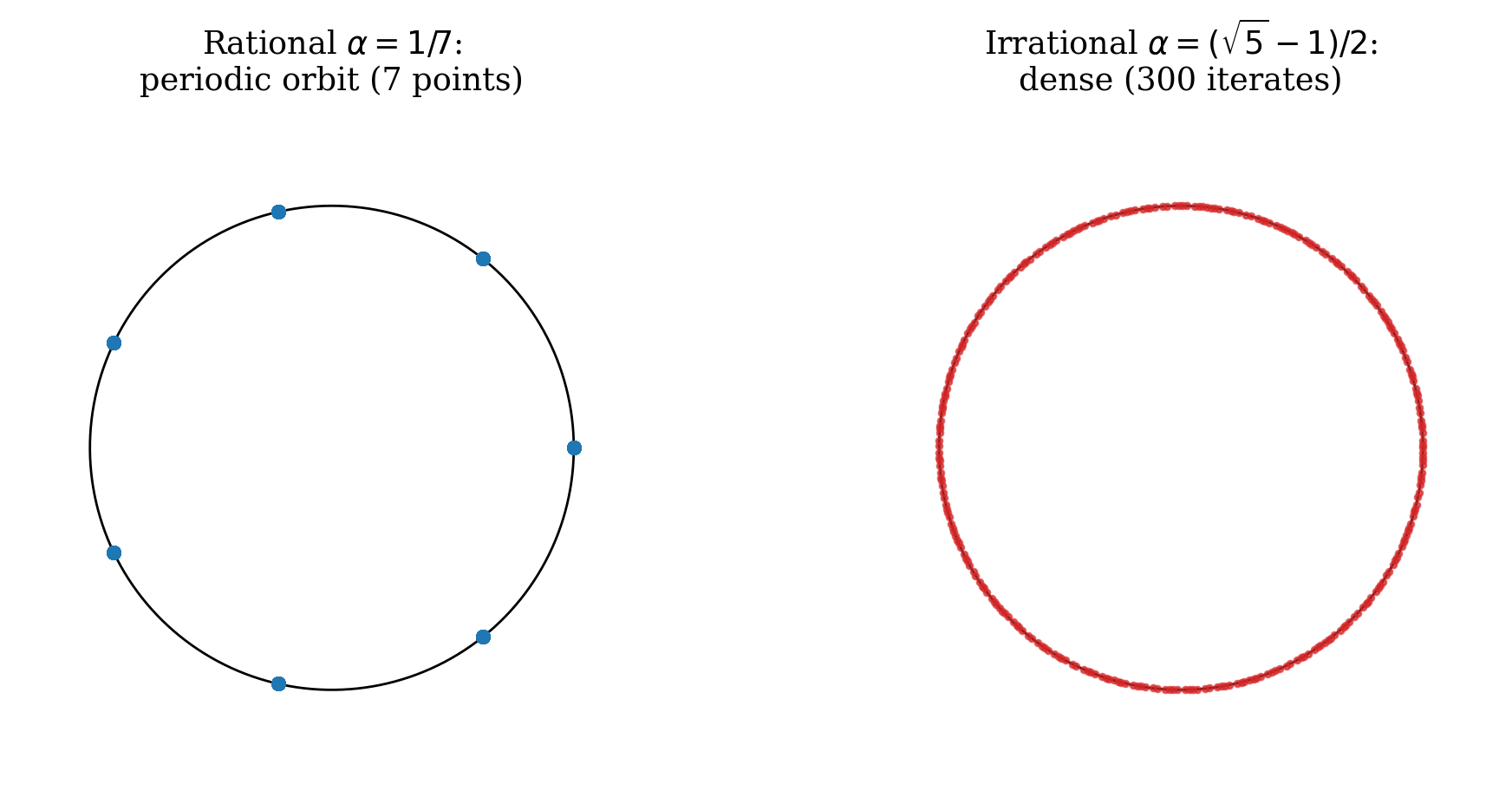
1. The space is $X=[0,1]$ (mod 1), with the Borel $\sigma$-algebra and the Lebesgue measure $\mu$. The dynamics are given by the map $x \mapsto x + \alpha$.
2. Same space as above, but we further restrict $\alpha=p/q$ to be rational, and the measure $\mu$ to be the uniform measure on the points $\left\{\frac{n}{q} : n \in \mathbb{N}\right\}$.
3. The space is $S^1 = \{e^{i\theta}\}$, with dynamics given by $z \mapsto \alpha z$, where $\lvert\alpha\rvert=1$. The measure is the Lebesgue measure on the angle coordinate.
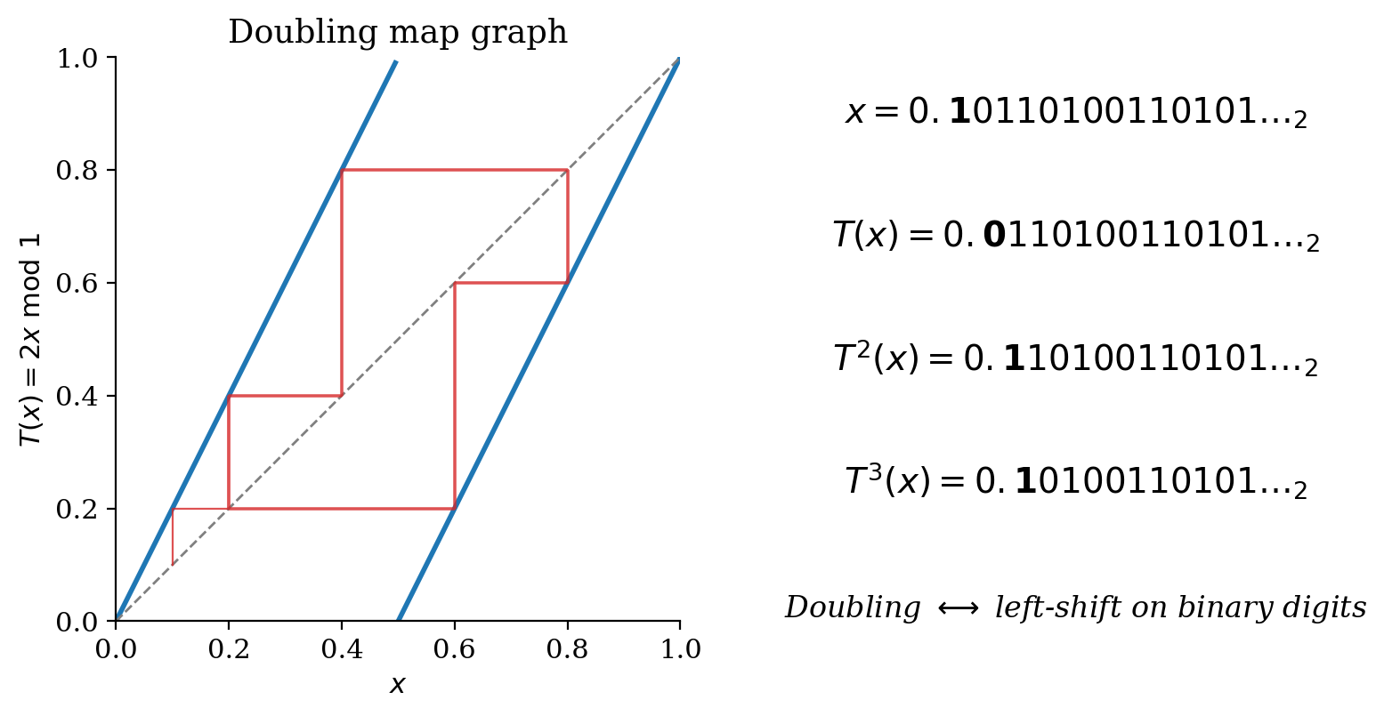
4. The space is $X=[0,1]$ (mod 1), with the Borel $\sigma$-algebra and the Lebesgue measure $\mu$. The dynamics are given by the map $x \mapsto 2x$. This is known as the doubling map.
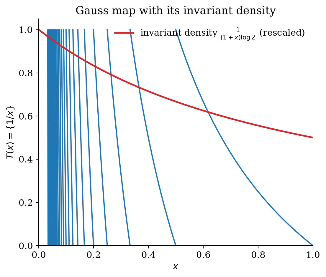
5. The space is $X=(0,1]$, with the Borel $\sigma$-algebra and the measure $d\mu = \frac{dx}{x+1}$. The map $T$ is given by $x \mapsto \frac{1}{x} - \left\lfloor \frac{1}{x} \right\rfloor$. This is known as the Gauss map.

Verification of invariance.

1. Define a new measure $\nu(A) = \mu(T^{-1}(A))$ to be the “pushforward” of the previous measure under the dynamics. Then, our claim reduces to showing $\nu = \mu$. For any two finite Borel measures, it suffices to check they agree on intervals (which generate the Borel $\sigma$-algebra). Consider an interval $I = (a,b)$. Then, $\mu(I) = b-a$. To compute $\nu(I) = \mu(T^{-1}(I))$, we need to find the preimage of $I$ under the rotation map $T(x) = x + \alpha \pmod{1}$. We do casework based on whether the interval wraps around. In all cases, the total measure is $b-a$, so $\nu(I) = \mu(I)$.

2. We write the Dirac measure at a point $x_0$ as $\mu_{x_0}(A) = 1$ if $x_0 \in A$, else $0$. Then, the given measure is $\frac{1}{q}\sum_{i=0}^{q-1} \mu_{i/q}$. Under the rotation $T(x) = x + p/q$, the set of points $\{0, 1/q, 2/q, \ldots, (q-1)/q\}$ is permuted cyclically, so the measure is invariant.

3. This system is isomorphic to system (1), by letting $\alpha’ = \arg(\alpha)/2\pi$.

4. We will check that $\int f(T(x))\, d\mu = \int f\, d\mu$ as follows. We know that $T(x) = \frac{1}{x} - n$ if $x \in \left(\frac{1}{n+1}, \frac{1}{n}\right]$.

   \[\begin{aligned} \int f(T(x))\, d\mu &= \int_0^1 f(T(x))\, \frac{dx}{x+1} \\ &= \sum_{n=1}^\infty \int_{1/(n+1)}^{1/n} f(T(x))\, \frac{dx}{x+1} \\ &= \sum_{n=1}^\infty \int_{1/(n+1)}^{1/n} f\!\left(\frac{1}{x} - n\right)\, \frac{dx}{x+1} \end{aligned}\]

   Setting $u = \frac{1}{x} - n$, we get

   \[\begin{aligned} \int f(T(x))\, d\mu &= \sum_{n=1}^\infty \int_0^1 \frac{f(u)\, du}{(u+n)(u+n+1)} \\ &= \sum_{n=1}^\infty \int_0^1 \left( \frac{f(u)}{u+n} - \frac{f(u)}{u+n+1} \right) du \\ &= \int_0^1 \sum_{n=1}^\infty \left( \frac{f(u)}{u+n} - \frac{f(u)}{u+n+1} \right) du \\ &= \int_0^1 \frac{f(u)\, du}{u+1} \\ &= \int f\, d\mu \end{aligned}\]

   which shows that this is an invariant measure. This example has deep connections to the math of continued fractions and number theory. $\blacksquare$

I’d like to do one other example separately: the construction here ends up being quite useful to understand the connections between dynamical systems and probability theory, especially that of Markov chains.

Example 1.3 (Shift maps on a sequence space). Given a finite list of $n+1$ symbols $[n] = \{0, 1, \ldots, n\}$, we define the space to be $X = [n]^\mathbb{N}$, the set of infinite sequences with these symbols. To construct a measure on this space, we start with a probability vector $(p_0, p_1, \ldots, p_n)$ and the associated measure $\nu = \sum_{j=0}^n p_j \delta_{\{j\}}$ on $[n]$. Then, we can construct the product $\sigma$-algebra $\Sigma$ on $X$, which is generated by the so-called cylinder sets: sets of the form $A = A_0 \times A_1 \times \cdots \times A_k \times [n] \times [n] \times \cdots$, where $A_0, A_1, \ldots, A_k \subseteq [n]$. We can use $\nu$ to define a measure $\mu$ on $(X, \Sigma)$ by setting $\mu(A) = \nu(A_0)\nu(A_1)\cdots\nu(A_k)$ for any cylinder set $A$, and extending this to the entire algebra. This is a uniquely determined probability measure, by some standard measure theory.

The dynamics are then given by the left shift map $\tau$, which maps a sequence $(x_0, x_1, x_2, \ldots) \mapsto (x_1, x_2, x_3, \ldots)$. This is a measurable map, since for any cylinder set $A = A_0 \times A_1 \times \cdots \times A_k \times [n] \times [n] \times \cdots$, we have that $\tau^{-1}(A) = [n] \times A_0 \times A_1 \times \cdots \times A_k \times [n] \times [n] \times \cdots \in \Sigma$. Moreover, it is measure-preserving, since $\mu(\tau^{-1}(A)) = \nu([n])\mu(A) = \mu(A)$ by definition. This particular construction is known as a one-sided Bernoulli shift. Replacing $\mathbb{N}$ with $\mathbb{Z}$ yields the two-sided Bernoulli shift, and we can introduce some more subtlety into the given construction to accommodate more general Markov chains on $[n]$, or on arbitrary, non-finite state spaces.

It is also worth noting that in the case where $[n] = \{0,1\}$ and the probability vector is chosen to be uniform, i.e., $p_0 = p_1 = \frac{1}{2}$, the given system is isomorphic to Example 1.2(4) from the previous section, with the isomorphism given by expanding a number in its binary expansion (which is unique except for dyadic rationals, a set of measure 0). Doubling corresponds exactly to shifting the binary expansion of a number to the left by one place.

Theorem 1.4 (Poincaré Recurrence). Given a measure-preserving dynamical system $(X, \mathcal{X}, \mu, T)$ with $\mu$ finite, for any set $E \in \mathcal{X}$, the set of points

has measure zero.

In other words, for any set, almost all points return to the set under the dynamics. In fact, we can upgrade this even further and say that almost all points return infinitely often. The proof will make this clearer.

Proof. Let $E$ be a measurable set in $\mathcal{X}$ of positive measure. Let $A$ be the subset of points that do not recur, i.e., $A = \{x \in E : T^n(x) \notin E \text{ for all } n>0\}$.

Consider $T^{-n}(A)$ for $n > 0$. We have $\mu(T^{-n}(A)) = \mu(A)$ for all $n>0$ since the transformation is measure-preserving.

Also, note that if $m > n$, we have $T^{-n}(A) \cap T^{-m}(A) = \emptyset$. To see this, assume otherwise: suppose there exists $y \in T^{-n}(A) \cap T^{-m}(A)$. Then, $T^n(y), T^m(y) \in A$. But this implies that $T^{m-n}(T^n(y)) \in E$ (since $T^m(y) \in E$). However, this cannot be the case unless $m = n$, since $T^n(y) \in A$ and points in $A$ do not recur.

Now, since all the preimages are in the measure space $X$, we have

However, by disjointness,

Since this sum must be finite, we must have $\mu(A) = 0$. $\blacksquare$

Furthermore, we can strengthen this to prove that almost all points recur infinitely often. Let $A$ be the set of points that recur only finitely often. Then,

We define the set $A_0 = \{x \in E : T^m(x) \notin E \text{ for all } m > 0\}$ and further define $A_n = \{x : T^n(x) \in E,\ T^m(x) \notin E \text{ for all } m > n\}$ for $n \geq 1$.

We can check that $A_n = T^{-n}(A_0)$. If $x \in A_n$, we have that $T^{m-n}(T^n(x)) \notin E$ for all $m > n$, so $T^n(x) \in A_0$.

Thus, we can write $A \subseteq \bigcup_{k \geq 0} A_k$. But we know the $A_k$ are pairwise disjoint preimages of $A_0$, so by the above proof they must have measure 0. Thus, $A$ has measure zero, and therefore almost all points are infinitely recurrent.

Corollary 1.5 (Monkeys on a typewriter). A monkey typing randomly on a typewriter will eventually produce the entire works of Shakespeare.

Proof. Consider the finite set $L$ given by the 26 characters of the English alphabet and punctuation on a typewriter. Consider a probability vector $p$ on $L$ which is the probability that a given key is hit by the monkey, assumed to be independent of previous keystrokes. Then, construct the product space $L^\mathbb{N}$ as in the example of the Bernoulli shift. Then, the left shift map can be seen as “generating” text according to the probability distribution $p$. The subset of infinite sequences that begin with the entire works of Shakespeare is a subset of positive measure, and therefore the Poincaré recurrence theorem proves that a monkey typing forever will eventually type the entire works of Shakespeare. $\blacksquare$

Interpreting the Poincaré recurrence theorem is quite an interesting philosophical and mathematical question. We will not pursue it further here.

We are interested in the study of ergodic theory, so it seems only fair to define what we mean by ergodic. Note that there are a number of equivalent characterizations, some of which we will see below.

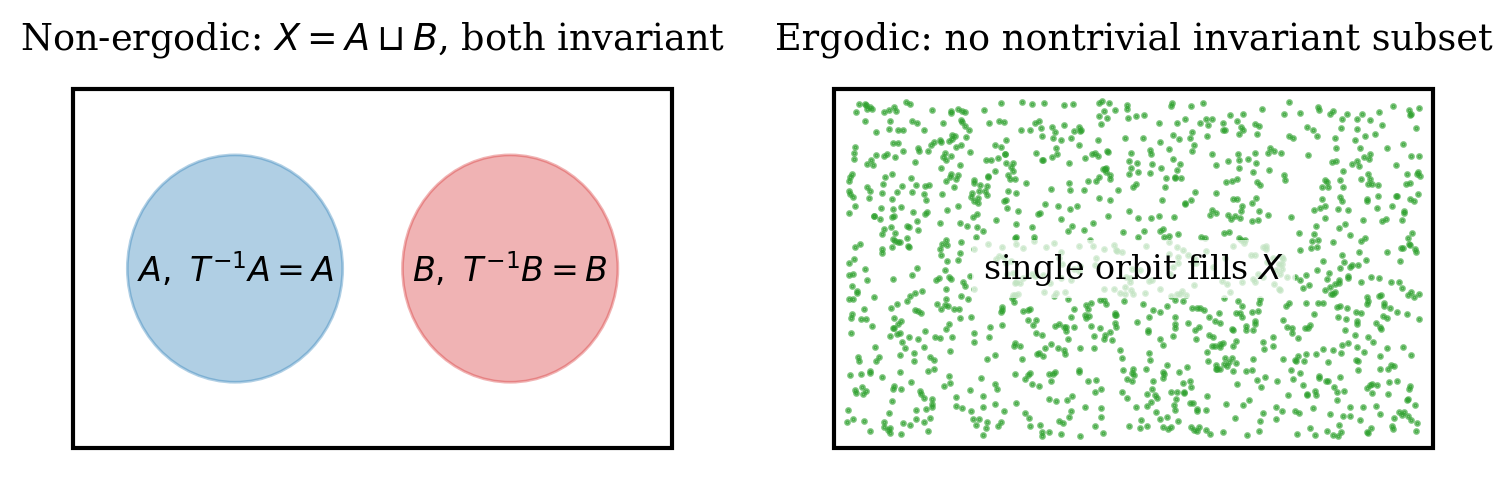
Definition 1.6. A measure-preserving dynamical system $(X, T, \mu)$ is said to be ergodic if, for any invariant set $S$ (i.e. $T^{-1}(S) = S$), we have $\mu(S) = 0$ or $1$.

Now, we can see some equivalent characterizations:

Theorem 1.7. The following are equivalent:

1. $(X, T, \mu)$ is ergodic.
2. $\mu(T^{-1}(S)\, \Delta\, S) = 0 \implies \mu(S) = 0$ or $1$.
3. If $\mu(S) > 0$, then $\mu!\left(\bigcup_{k>0} T^{-k}(S)\right) = 1$.
4. If $\mu(R) > 0$ and $\mu(S) > 0$, then there exists $n$ such that $\mu(T^{-n}(R) \cap S) > 0$.

Proof.

(1) $\Rightarrow$ (2): Let $B \subset X$ satisfy $\mu(T^{-1}B\, \Delta\, B) = 0$. We will construct a set $B_\infty$ such that $T^{-1}B_\infty = B_\infty$. Note that for any $n > 0$, we have

Thus, $\mu(T^{-n}B\, \Delta\, B) \leq n\mu(T^{-1}B\, \Delta\, B) = 0$. Now, define

By the above calculation,

Thus, $\mu(B_\infty\, \Delta\, B) = 0$, which implies $\mu(B_\infty) = \mu(B)$. Also, $B_\infty$ is invariant, since

This implies that either $\mu(B_\infty) = 0$ or $1$, which implies $\mu(B) = 0$ or $1$.

(2) $\Rightarrow$ (3): Consider the set $A = \bigcup_{k>0} T^{-k}(S)$. Then $T^{-1}(A) \subseteq A$, and $\mu(T^{-1}(A)) = \mu(A)$ since $T$ is measure-preserving, so $\mu(A \setminus T^{-1}(A)) = 0$, giving $\mu(A\, \Delta\, T^{-1}(A)) = 0$. By (2), $\mu(A) = 0$ or $1$. But if $\mu(S) > 0$, we have $S \subseteq A$, and so $\mu(A) = 1$.

(3) $\Rightarrow$ (4): Assume no such $n$ exists, i.e., $\mu(T^{-n}(R) \cap S) = 0$ for all $n$. Then,

But by hypothesis, $\mu!\left(\bigcup_{k>0} T^{-k}(R)\right) = 1$ and $\mu(S) > 0$. The intersection of a positive-measure set with a set of full measure must have positive measure, and thus this is a contradiction.

(4) $\Rightarrow$ (1): Suppose $B \subseteq X$ and $T^{-1}B = B$. If $0 < \mu(B) < 1$, then

for all $n \geq 1$, which contradicts (4). $\blacksquare$

Ergodicity should be understood as a sort of irreducibility criterion: there is no way to break our state space into two nontrivial subspaces that are invariant under the dynamics.

2. The Koopman Operator

Along with the invariant measure, we can look at the function spaces associated with it. A function $X \to \mathbb{C}$ is known as an observable, so these spaces are sometimes referred to as spaces of observables. Most commonly, we will study the Hilbert space of observables: $L^2(\mu)$, where the inner product is given by $\langle f, g \rangle = \int f\, \overline{g}\, d\mu$.

Definition 2.1. The Koopman operator is an operator $U: L^2(\mu) \to L^2(\mu)$ given by $Uf = f \circ T$.

We can check some basic features of the Koopman operator.

Theorem 2.2. The Koopman operator is continuous and an isometry of Banach spaces.

Proof. We have

But, since $\mu$ is invariant under the dynamics $T$, we can do a change of variables and see that $\int \lvert f \circ T \rvert^2\, d\mu = \int \lvert f \rvert^2\, d\mu$. Thus, $\lVert Uf \rVert = \lVert f \rVert$, i.e., it is an isometry. Also, $\lVert U \rVert = 1$, so it is bounded, and therefore continuous. $\blacksquare$

Also, note that the Koopman operator acts multiplicatively, i.e., $U(fg) = (Uf)(Ug)$.

In the Hilbert space setting, we have a few extra properties:

Theorem 2.3. If the dynamics $T$ are invertible, the Koopman operator $U: L^2(\mu) \to L^2(\mu)$ is a unitary operator.

Proof. Since $T$ is invertible, we have $U_T^{-1} = U_{T^{-1}}$. Then, consider

We can do a change of variables such that $y = T(x)$. Then $d\mu(y) = d\mu(x)$ since $\mu$ is invariant under $T$. Thus, the above equation becomes

Thus, we see that $U_T^\ast = U_T^{-1} = U_{T^{-1}}$, and thus the Koopman operator is unitary. $\blacksquare$

This gives us a new spectral characterization of ergodicity:

Theorem 2.4. $T$ is ergodic if and only if $U_T$ has a simple eigenvalue at $1$; equivalently, the only eigenfunction with eigenvalue $1$ is the constant function.

Proof.

($\Rightarrow$) Assume $T$ is ergodic. Suppose $f \in L^2(\mu)$ satisfies $U_T f = f$, i.e., $f \circ T = f$ almost everywhere. We need to show that $f$ is constant almost everywhere.

Let $R \subseteq \mathbb{R}$ be the range of $f$. We can split this into countably many intervals $I_k$ and consider the preimage

Since $f \circ T = f$ a.e., the function $f$ is $T$-invariant. By the $T$-invariance of $f$, we have $T^{-1}(A_k) = A_k$ up to measure zero. That is, $A_k$ is $T$-invariant.

Since $T$ is ergodic, every $T$-invariant set has measure $0$ or $1$. Therefore, for each $k \in \mathbb{N}$, either $\mu(A_k) = 0$ or $\mu(A_k) = 1$.

Since the total measure of the space is $1$, and $X = \bigcup_{k \in \mathbb{N}} A_k$, there can be at most one value $k_0$ with $\mu(A_{k_0}) = 1$. Thus the function takes values in $I_{k_0}$. But we can further subdivide $I_{k_0}$ into $2^{k’}$ intervals, and repeat the same argument. Thus, we see that the diameter of the range of $f$ is at most $2^{-n}$ for any $n > 0$, and thus the function must be constant almost everywhere.

($\Leftarrow$) Now, assume $T$ is not ergodic. Then there exists a set $S$ such that $T^{-1}(S) = S$ and $0 < \mu(S) < 1$. Consider the characteristic function $\chi_S$. Then $U \chi_S = \chi_S$ since $S = T^{-1}(S)$. Thus $\chi_S$ is a non-constant eigenfunction with eigenvalue 1. $\blacksquare$

This allows us to prove the ergodicity of some basic examples using Fourier theory.

Examples 2.5.

1. Consider the rotation map on $S^1 = \{e^{i\theta}\}$, with dynamics given by $z \mapsto \alpha z$ where $\lvert\alpha\rvert = 1$. The measure is Haar measure (Lebesgue measure on the angle). This dynamical system is ergodic if and only if $\alpha$ is not a root of unity.
2. Consider the doubling map on $S^1$, $z \mapsto z^2$, with the Haar measure. This map is ergodic.

Proof.

1. If $\alpha$ is a root of unity such that $\alpha^p = 1$, consider the function $f(z) = z^p$. This is not a constant function, but is an eigenfunction with eigenvalue 1, since

   \[Uf = f \circ T = f(\alpha z) = (\alpha z)^p = \alpha^p z^p = z^p = f.\]

   Now, assume $\alpha$ is not a root of unity. Consider a function such that $Uf = f$. We know $f$ has a Fourier series expansion $f(z) = \sum_{n=-\infty}^\infty c_n z^n$. Then, $Uf(z) = f(\alpha z) = \sum_{n=-\infty}^\infty c_n (\alpha z)^n = \sum_{n=-\infty}^\infty c_n \alpha^n z^n$. Matching coefficients, we get $c_n = \alpha^n c_n$ for all $n$. This is only possible if $\alpha^n = 1$ or $c_n = 0$. Since $\alpha$ is not a root of unity, $\alpha^n \neq 1$ for $n \neq 0$, so $c_n = 0$ for all $n \neq 0$. Therefore, $f$ is the constant function.

2. For the doubling map, we again assume $f(z) = \sum_{n=-\infty}^\infty c_n z^n$ is an eigenfunction such that $Uf = f$. Then,

   \[Uf = \sum_{n=-\infty}^\infty c_n (z^2)^n = \sum_{n=-\infty}^\infty c_n z^{2n}.\]

   Matching coefficients, we see that $c_n = c_{2n}$ for all $n$. But we must have $\sum_n \lvert c_n \rvert^2 < \infty$ (since $f \in L^2$), and thus $c_n = 0$ for all $n \neq 0$. Thus, the function is constant. $\blacksquare$

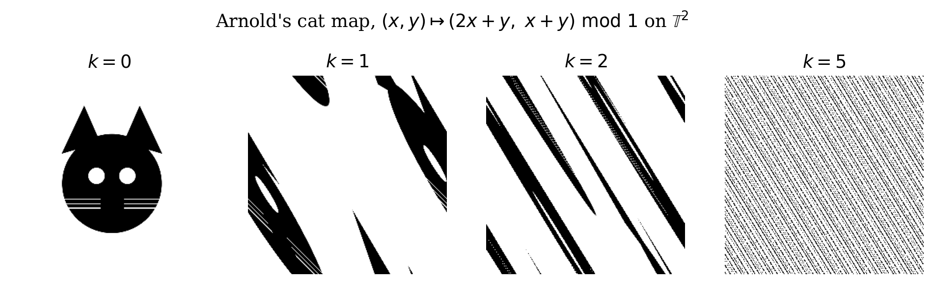
It is worth noting that the above proof can be applied in slightly more generality to the case of toral automorphisms. We state it here for completeness, without proof.

If $A \in \mathrm{GL}_n(\mathbb{Z})$, then it induces a map $\mathscr{T}_A : \mathbb{T}^n \to \mathbb{T}^n$ preserving the Lebesgue measure induced on $\mathbb{T}^n = \mathbb{R}^n / \mathbb{Z}^n$ by noting that the action of $A: \mathbb{R}^n \to \mathbb{R}^n$ preserves $\mathbb{Z}^n$. These are the toral automorphisms.

Theorem 2.6. $\mathscr{T}_A$ is ergodic if and only if no eigenvalue of $A$ is a root of unity.

If a toral automorphism has no eigenvalues of modulus $1$, we say it is a hyperbolic automorphism. People like studying these.

The next theorem proves some basic spectral properties of the Koopman operator, which end up being quite useful.

Theorem 2.7. Let $T$ be a measure-preserving transformation of $(X, \mathcal{X}, \mu)$, and suppose $T$ is ergodic. Then, the following are true:

1. If $Uf = \lambda f$ for some $f \in L^2(\mu)$, $f \neq 0$, then $\lvert\lambda\rvert = 1$ and $\lvert f \rvert$ is constant a.e.
2. Eigenfunctions corresponding to different eigenvalues are orthogonal.
3. The eigenvalues form a subgroup of the unit circle.

Proof.

1. We have $\lVert Uf \rVert = \lvert\lambda\rvert \lVert f \rVert$, so $\lVert f \rVert = \lvert\lambda\rvert \lVert f \rVert$, which implies $\lvert\lambda\rvert = 1$. Then, we know $U\lvert f\rvert = \lvert f \circ T \rvert = \lvert \lambda f \rvert = \lvert\lambda\rvert \lvert f\rvert = \lvert f\rvert$, and thus by ergodicity, $\lvert f\rvert$ is constant almost everywhere.

2. Let $Uf = \alpha f$ and $Ug = \beta g$, with $\alpha \neq \beta$. Then,

   \[\langle f, g \rangle = \langle Uf, Ug \rangle = \langle \alpha f, \beta g \rangle = \alpha \overline{\beta} \langle f, g \rangle.\]

   Thus, we must either have $\alpha = \beta$ or $\langle f, g \rangle = 0$.

3. Let $Uf = \alpha f$ and $Ug = \beta g$. Then,

   \[U(f\overline{g}) = (f\overline{g}) \circ T = (f \circ T)\cdot(\overline{g} \circ T) = (\alpha f)\cdot(\overline{\beta g}) = \alpha \overline{\beta} f \overline{g}\]

   This implies that $\alpha \overline{\beta}$ is also an eigenvalue, and therefore the eigenvalues form a subgroup. $\blacksquare$

3. Ergodic Theorems

Boltzmann’s ergodic hypothesis asks when averaging an observable over time under some dynamics (a time mean) equals a spatial average over the entire space. In mathematical language, he asks first: when, given an observable $f$ on a state space $X$ and an initial condition $x_0$, does the time average

converge and become independent of the initial condition? Moreover, he asks when this equals $\int f\, d\mu$, the spatial average of the function over the state space. This question was first answered by von Neumann in a Hilbert-space sense, and then generalized by Birkhoff in a pointwise sense.

Theorem 3.1 (von Neumann Mean Ergodic Theorem). Let $\mathrm{fix}(T)$ denote the observables that are invariant under the dynamics, i.e., the eigenspace associated to the eigenvalue 1 of the Koopman operator $U$. Furthermore, let $P$ denote the orthogonal projection onto this closed subspace. Then, for any observable $f \in L^2(\mu)$, we have

in the $L^2$ norm.

We give the slick proof by Riesz. Before that, note that if $U$ is unitary and $Uv = v$, we have $U^\ast v = U^\ast Uv = Iv = v$.

Proof. The statement is trivially true for $f \in \mathrm{fix}(T)$. Let $W$ be the subspace of vectors that can be written as $Uw - w$ for some $w \in H$. Then, given $v \in \mathrm{fix}(T)$ and $w \in H$, we have

where we used the fact that $U^{\ast}v = v$ (since $v$ is invariant and $U$ is an isometry). Thus $W \perp \mathrm{fix}(T)$, and in particular, $P(Uw - w) = 0$. Furthermore, the sum $\frac{1}{N} \sum_{n=0}^{N-1} U^n(Uw - w)$ telescopes: we have

Taking norms, we see that

Thus, the statement is true on $\mathrm{fix}(T)$ and $W$, and thus by linearity on $W + \mathrm{fix}(T)$.

Now, we need to extend this from $\mathrm{fix}(T) + W$ to $\overline{\mathrm{fix}(T) + W}$. To do this, note that the linear transformation $A_N: v \mapsto \frac{1}{N} \sum_{n=0}^{N-1} U^n v$ is uniformly bounded, since

Thus, by the bounded linear transformation theorem, $\lim_{N \to \infty} A_N$ uniquely extends to a bounded linear transformation on all of $\overline{\mathrm{fix}(T) + W}$, and the given property holds by continuity.

To see that $\overline{\mathrm{fix}(T) + W}$ is the entire space $H$, assume that there is a vector $g \in (\mathrm{fix}(T) + W)^\perp$. Then, in particular, $g \perp Uf - f$ for all $f \in H$. Now, this implies that

But this is true for all $f$, and hence $U^\ast g - g = 0$. Since $U$ is unitary, this implies $Ug = g$. Thus $g \in \mathrm{fix}(T)$, contradicting $g \perp \mathrm{fix}(T)$ unless $g = 0$. Therefore, $\overline{\mathrm{fix}(T) + W} = H$.

The convergence for general $f \in H$ follows by approximation. $\blacksquare$

Note that if $T$ is ergodic, the space $\mathrm{fix}(T)$ is one-dimensional and comprises only the constant functions by Theorem 2.4.

Note that the convergence in Theorem 3.1 is in an $L^2$ norm. We can upgrade this convergence to pointwise almost-everywhere convergence in the following generalization by Birkhoff:

Theorem 3.2 (Birkhoff Pointwise Ergodic Theorem). For $f \in L^1(\mu)$, the limit

exists for almost every $x \in X$. Moreover, if $T$ is ergodic, then this limit equals $\int f\, d\mu$ for almost every $x$.

Before we prove this, let us first note some interesting consequences of this theorem. Firstly, this implies the von Neumann ergodic theorem, since pointwise almost-everywhere convergence of $L^1$ functions implies convergence in $L^2$ norm.

Second, as an application, here is yet another equivalent definition of ergodicity:

Theorem 3.3. A measure-preserving dynamical system $(X, \mathcal{X}, \mu, T)$ is ergodic if and only if for any two $A, B \in \mathcal{X}$, we have

Proof. First, assume $T$ is ergodic. Then, applying the Birkhoff ergodic theorem to $f = \chi_A$ gives us that $\lim_{N \to \infty} \frac{1}{N} \sum_{n=0}^{N-1} U^n(\chi_A)(x) = \mu(A)$. We can then multiply both sides by $\chi_B$ and integrate to see the statement holds.

Now, assume the statement holds, and $E = T^{-1}(E)$. Apply the convergence statement for $A = B = E$, and we see that $\mu(E) = \mu(E)^2$, which implies that $\mu(E) = 0$ or $1$. $\blacksquare$

Lastly, it is worth noting that this gives a concrete mathematical foundation for Boltzmann’s ergodic hypothesis, which is informally stated as “time mean equals space mean” in the limit. Given an observable $f$ with initial condition $x$, the time average of this observable is given by $\frac{1}{N}\sum_{n=0}^{N-1} U^n f(x) = \frac{1}{N}\sum_{n=0}^{N-1} f(T^n(x))$. The average over the phase space is given by $\int f\, d\mu$, which is independent of the initial condition. Birkhoff’s ergodic theorem is the statement that in the large-time limit, these two are equal.

Lastly, we present a rather famous application of this to number theory.

Theorem 3.4 (Borel Theorem on Normal Numbers). Almost all numbers in $[0,1)$ are normal to base 2, that is, the proportion of $1$s in the binary expansion of numbers is $1/2$.

Proof. As noted earlier, almost all numbers have a unique binary representation. Then, consider $f = \chi_{[1/2, 1)}(x)$, the characteristic function of the interval $[1/2, 1)$. Then, $f(T^i(x))$ is $1$ if the $(i+1)$-th digit in its binary expansion is $1$, and $0$ otherwise. Thus, we see that $\frac{1}{N}\sum_{n=0}^{N-1} f(T^n(x))$ is the proportion of $1$s in the binary expansion in the first $N$ digits. By the pointwise ergodic theorem, we know that this converges in large $N$ to $\int f\, d\mu = \mu([1/2, 1)) = \frac{1}{2}$. This proves the given result. $\blacksquare$

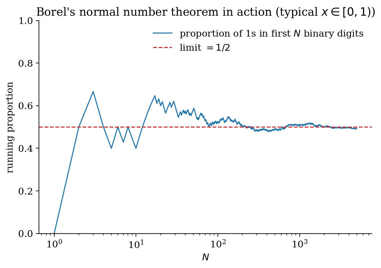
Since the countable union of measure-zero sets is measure zero, this can easily be extended to proving that almost all numbers are absolutely normal, i.e., normal in every base.

There are countless proofs of Birkhoff’s theorem, and none of them are particularly easy. Most of them use some type of maximal inequality to show the existence of the pointwise limit, and ergodicity to show that it converges to what it must be. We will only prove the case where $T$ is ergodic and $f \in L^\infty$.

Proof. WLOG, we will deal with real-valued positive functions, since we can always handle the real and complex parts separately, as well as the positive and negative parts separately. Furthermore, since we assume $f$ is essentially bounded, we can rescale $f’ = \frac{f}{\lVert f \rVert_\infty}$ so that $f’ \leq 1$.

Let $A_N f = \frac{1}{N}\sum_{n=1}^N f \circ T^n$. Let $f_+(x) = \limsup_N A_N f(x)$ and $f_-(x) = \liminf_N A_N f(x)$. It suffices to show that for any $\varepsilon > 0$, we have that $f_+(x) < \int f\, d\mu + \varepsilon$ for almost all $x$, since we can then apply the same argument to $g = 1 - f$ to get an estimate for $f_-$.

Now, let $B = \{x : f_+(x) \geq \int f\, d\mu + \varepsilon\}$. Clearly $T^{-1}(B) = B$, so by ergodicity, we must have $\mu(B) = 0$ or $1$. We will show $\mu(B) < 1$, and therefore $\mu(B) = 0$, which is sufficient.

Now, let $\alpha = \int f\, d\mu + \varepsilon$ and let $f_n(x) = f(x) + f(T(x)) + \cdots + f(T^{n-1}(x)) - n\alpha$, and let $F_N = \max\{0, f_1, f_2, \ldots, f_N\}$. Let $B_N$ denote the set $\{x \in X : F_N(x) > 0\}$. Then, clearly, for $x \in B_{N+1}$, for $n \leq N$, we have that $F_N(x) \geq f_n(x)$, and so $F_N(Tx) \geq f_n(Tx)$. This further implies that $F_N(Tx) + f(x) \geq f_n(Tx) + f(x) = f_{n+1}(x) + \alpha$. Taking a maximum over all $n$, we see that

We can integrate this over $B_{N+1}$ to see that

Thus, we see that

But we know that $B_N \subseteq B_{N+1}$, so these sets are nested, and thus we have that

Also, we see that the set $\{x \in X : f_n(x) > 0 \text{ infinitely often}\} \subseteq \bigcup_{N>0} B_N$. But this is simply the set $B$, and therefore $\mu(B) < 1$. This completes the proof. $\blacksquare$

4. Mixing

Mixing (and the associated notion of weak mixing) are a strengthening of ergodicity. We showed in Section 3 that a dynamical system $(X, T, \mu)$ is ergodic if and only if for any two sets $A, B \subseteq X$, we have

This allows us to generalize the notion of convergence and define mixing as follows.

Definition 4.1. For a measure-preserving dynamical system $(X, \mathcal{X}, \mu, T)$ and any two $A, B \in \mathcal{X}$:

1. $T$ is weak-mixing if

   \[\lim_{N \to \infty} \frac{1}{N} \sum_{n=0}^{N-1} \lvert \mu(T^{-n}(A) \cap B) - \mu(A)\mu(B) \rvert = 0.\]

2. $T$ is (strong) mixing if

   \[\lim_{n \to \infty} \mu(T^{-n}(A) \cap B) = \mu(A)\mu(B).\]

Clearly, strong mixing implies weak mixing, which implies ergodicity.

It is fairly easy to check (and we will do so shortly) that the rotation map $z \mapsto \alpha z$ is ergodic but not weak-mixing (when $\alpha$ is not a root of unity). An example of a map that is weak-mixing but not strong-mixing is somewhat more difficult to give explicitly, but an example of this was given by Chacon (1969) using a cutting-and-stacking argument [3].

An additional characterization of properties such as ergodicity and mixing comes from the decay-of-correlations perspective. We define the correlation of two observables $f, g \in L^2(\mu)$ at time $t$ to be given by the correlation function $C_t(f, g) = \langle U^t f, g \rangle = \int (U^t f) \overline{g}\, d\mu$.

We can then write the following characterization of ergodicity, weak-mixing, and strong-mixing:

Theorem 4.2. Suppose $(X, \mathcal{X}, \mu, T)$ is a measure-preserving dynamical system, with $U$ the associated Koopman operator. The following are true:

1. $T$ is ergodic if and only if for all $f, g \in L^2(\mu)$

   \[\lim_{N \to \infty} \frac{1}{N} \sum_{n=0}^{N-1} \langle U^n f, g \rangle = \langle f, 1 \rangle \langle 1, g \rangle.\]

2. $T$ is weak-mixing if and only if for all $f, g \in L^2(\mu)$,

   \[\lim_{N \to \infty} \frac{1}{N} \sum_{n=0}^{N-1} \lvert \langle U^n f, g \rangle - \langle f, 1 \rangle \langle 1, g \rangle \rvert = 0.\]

3. $T$ is strong-mixing if and only if for all $f, g \in L^2(\mu)$,

   \[\lim_{n \to \infty} \langle U^n f, g \rangle = \langle f, 1 \rangle \langle 1, g \rangle.\]

Proof. I will show this only for weak-mixing, since all three proofs are fairly similar. In particular, I will show that the following are equivalent:

1. $T$ is weak-mixing.

2. For all $f, g \in L^2(\mu)$,

   \[\lim_{N \to \infty} \frac{1}{N} \sum_{n=0}^{N-1} \lvert \langle U^n f, g \rangle - \langle f, 1 \rangle \langle 1, g \rangle \rvert = 0.\]

3. For all $f \in L^2(\mu)$,

   \[\lim_{N \to \infty} \frac{1}{N} \sum_{n=0}^{N-1} \lvert \langle U^n f, f \rangle - \langle f, 1 \rangle \langle 1, f \rangle \rvert = 0.\]

4. For all $f \in L^2(\mu)$,

   \[\lim_{N \to \infty} \frac{1}{N} \sum_{n=0}^{N-1} \lvert \langle U^n f, f \rangle - \langle f, 1 \rangle \langle 1, f \rangle \rvert^2 = 0.\]

Throughout, write

which is linear in $f$, conjugate-linear in $g$, and satisfies $\lvert c_n(f,g)\rvert \leq 2\lVert f\rVert \lVert g\rVert$, since $U$ is an isometry and $\lVert 1\rVert = 1$.

(2) $\Rightarrow$ (1): Set $f = \chi_A$, $g = \chi_B$. Then we have that

This shows $T$ is weak-mixing.

(2) $\Rightarrow$ (3): Set $f = g$.

(1) $\Rightarrow$ (2): Weak-mixing is exactly the statement for $f = \chi_A$, $g = \chi_B$. Since $c_n$ is sesquilinear, it extends to all simple $f, g$. For general $f, g \in L^2(\mu)$, fix $\varepsilon > 0$ and choose simple $h, k$ with $\lVert f - h\rVert < \varepsilon$ and $\lVert g - k\rVert < \varepsilon$. Then

so, using the uniform bound on $c_n$,

Averaging over $n < N$ and letting $N \to \infty$, the last term contributes nothing, so

As $\varepsilon$ was arbitrary, the limit is $0$.

(3) $\Leftrightarrow$ (4): Put $a_n = \lvert c_n(f,f)\rvert$, so $0 \leq a_n \leq C := 2\lVert f\rVert^2$. If (3) holds then $a_n^2 \leq C a_n$ gives $\frac{1}{N}\sum a_n^2 \leq C \cdot \frac{1}{N}\sum a_n \to 0$. Conversely, Cauchy–Schwarz gives $\bigl(\frac{1}{N}\sum a_n\bigr)^2 \leq \frac{1}{N}\sum a_n^2$, so (4) implies (3).

(3) $\Rightarrow$ (2): We use the following standard fact.

Lemma (Koopman–von Neumann). Let $(a_n)$ be a bounded sequence of nonnegative reals. Then $\frac{1}{N}\sum_{n<N} a_n \to 0$ if and only if there is a set $J \subseteq \mathbb{N}$ of density $1$ with $a_n \to 0$ as $n \to \infty$ along $J$.

Proof of the lemma. If such a $J$ exists, then given $\varepsilon > 0$ we have $a_n < \varepsilon$ for large $n \in J$, while the complement contributes at most $C$ times its density, which tends to $0$; so the averages are eventually below $2\varepsilon$. Conversely, let $J_k = \{n : a_n < 1/k\}$. From $\frac{1}{N}\sum a_n \geq \frac{1}{k}\cdot\frac{\lvert [0,N) \setminus J_k\rvert}{N}$ we see each $\mathbb{N} \setminus J_k$ has density $0$; choose $N_1 < N_2 < \cdots$ so that this density stays below $1/k$ beyond $N_k$, and set $J = \bigcup_k \bigl(J_k \cap [N_k, N_{k+1})\bigr)$. Then $J$ has density $1$ and $a_n \to 0$ along $J$. $\square$

Now let $f, g \in L^2(\mu)$, and assume without loss of generality that $\langle f,1\rangle = \langle g,1\rangle = 0$, so that $c_n(f,g) = \langle U^n f, g\rangle$. Apply (3) together with the lemma to each of $f$, $g$, $f+g$ and $f + ig$, and let $J$ be the intersection of the four resulting density-$1$ sets; a finite intersection of density-$1$ sets again has density $1$. Along $J$, all four of $\langle U^n f, f\rangle$, $\langle U^n g, g\rangle$, $\langle U^n(f+g), f+g\rangle$ and $\langle U^n(f+ig), f+ig\rangle$ tend to $0$. Expanding the third,

so $\langle U^n f, g\rangle + \langle U^n g, f\rangle \to 0$ along $J$. Expanding the fourth, and using $\langle x, iy\rangle = -i\langle x,y\rangle$ and $\langle ix, y\rangle = i \langle x,y\rangle$,

so $\langle U^n f, g\rangle - \langle U^n g, f\rangle \to 0$ along $J$. Adding the two gives $\langle U^n f, g\rangle \to 0$ along $J$, and the lemma applied in the other direction turns this back into

which is (2). Together with (2) $\Rightarrow$ (1) this closes the cycle. $\blacksquare$

Weak-mixing, in particular, lends itself to a characterization in terms of the eigenvalues and eigenfunctions of the Koopman operator.

Theorem 4.3. A system is weak-mixing if and only if it has a simple eigenvalue at 1 and no other eigenvalues.

Proof. Assume that the system is weak-mixing, and $\lambda \neq 1$ is an eigenvalue such that $Uf = \lambda f$. Then, we know that the quantity $\langle U^n f, f \rangle = \lambda^n \langle f, f \rangle$. Since $\lambda \neq 1$, we have that $\langle f, 1 \rangle = 0$ by orthogonality of eigenvectors. Also, we know that $\lvert\lambda\rvert = 1$ for all eigenvalues. Putting this together, we see that

by weak-mixing, which implies that $f$ is the zero function.

Now, assume that the system has no eigenvalues. Let $f$ be a fixed observable. Then, we can invoke the spectral theorem for unitary operators (or more generally bounded normal operators) to say that there exists a measure $\mu_f$ such that

To show the system is weak-mixing, it suffices to show that

Assume WLOG that $\langle f, 1 \rangle = 0$. Since we know that the eigenvalue at 1 is simple, we know that $f$ is in the orthogonal complement of the projection-valued measure onto $\{1\}$. Then, we can write

Now, if $\lambda \neq \tau$, we can write $\sum_{n=0}^{N-1} \lambda^n \overline{\tau}^n = \frac{(\lambda\overline{\tau})^N - 1}{(\lambda\overline{\tau}) - 1}$. But, since the measure $\mu_f$ has no atoms, the diagonal set $\{(\lambda, \lambda) \in S^1 \times S^1\}$ has 0 measure in the product measure $d(\mu_f \times \mu_f)(\lambda, \tau)$, and thus the following holds almost everywhere:

where we used the dominated convergence theorem in the last line to exchange the limit and the integral. $\blacksquare$

5. Advanced Results and Applications

5.1 Continuous-time Dynamical Systems

These notes are largely dedicated to studying discrete-time dynamical systems. It is possible to study the action of continuous-time dynamical systems, or even dynamical systems associated to the action of more general semigroups. To do this, we present a new definition of dynamical systems that highlights their connection to group actions.

Definition 5.1. A dynamical system is a triple $(X, G, \Phi)$ comprising a state space $X$, a semigroup $G$, and a map $\Phi: G \times X \to X$ which satisfies $\Phi(t+s, x) = \Phi(t, \Phi(s, x))$, which is known as the cocycle condition. Often, we write $\Phi(t, \cdot) = \Phi^t(x)$, in which case this notation simplifies to $\Phi^{t+s}(x) = \Phi^t \circ \Phi^s(x)$.

Note that in the case that $X$ is a measure space and $G$ is $\mathbb{N}$, we recover the case of discrete-time measurable dynamical systems. We can also use $G = \mathbb{R}$ to analyze the case of continuous-time dynamics. This perspective is quite flexible, and choosing $G$ to be a group other than $\mathbb{N}$, $\mathbb{Z}$, or $\mathbb{R}$ can often result in very interesting mathematics that I do not understand very well.

This formalism also lends itself to define random dynamical systems quite easily. In a random dynamical system, the dynamical map at each timestep is not a deterministic map, but rather randomly chosen according to some distribution. The trick here, then, is to expand our state space to include the randomness, and view it as a deterministic dynamical system on this space. Formally, let $\Omega= (\Omega, \mathcal{F}, P)$ be a probability space, known as the noise space, and let $X= (X, \Sigma, \mu)$ be our standard state space. On the noise space, we have a (measurable) flow $\theta: G \times \Omega \to \Omega$ which ‘evolves’ the noise. This must satisfy $\theta(0, \cdot) = \text{Id}$, and $\theta_{t+s} = \theta_t \circ \theta_s$. Then, a random dynamical system $\Phi$ is a measurable map $\Phi: G \times \Omega \times X \to X$ which satisfies the following cocycle condition:

This cocycle condition should be read as ‘evolving a random dynamical system for time $t+s$’ should be the same as ‘evolve a system for time $s$, followed by evolving it for time $t$ starting the noise at $s$’. This is a mouthful, so let’s look at a simple example.

Example 5.2 (Random rotations on a circle). We work in discrete time. We fix an angle $\alpha$, and at each time, we will flip a fair coin, and rotate clockwise or anticlockwise according to it.

In this example, since time is discrete, we fix our semigroup to be $G= \mathbb{N}$. Our state space $X=S^1$, which we write multiplicatively with the usual Haar measure and $\sigma$-algebra. Our noise space is our sequence of flips: the space is $\Omega = \{0,1\}^\mathbb{N}$, with the cylindrical Bernoulli measure we defined earlier. The noise evolution map $\theta$ is just given by the left-shift, and the dynamics are given by (for one time step), $\Phi(\omega, z) = \Phi(\theta(\omega), \exp(i(-1)^{\omega_0} \alpha) \cdot z)$. We can get the action at time $t$ by iterating this using the cocycle condition.

5.2 Fun Applications

Theorem 5.3 (Benford’s Law). Benford’s law is the observation that the distribution of first digits of numbers found in data, especially financial data, empirically follows the distribution below, with digit $d \in \{1, \ldots, 9\}$ occurring with probability $\log_{10}(1 + 1/d)$.

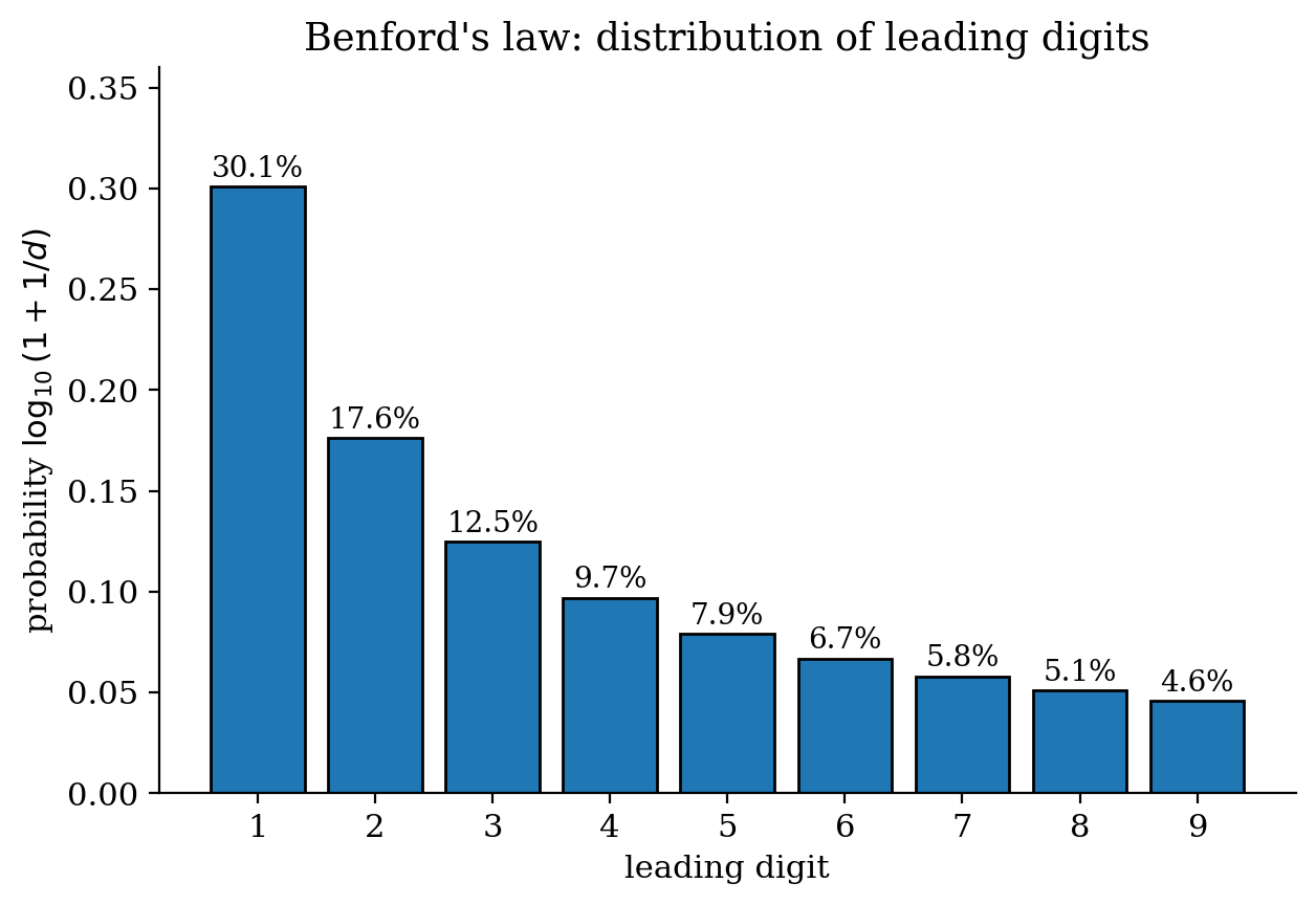
While this observation is largely empirical, it is mostly observed in datasets that contain numbers of various orders of magnitude: electricity bills, street addresses, stock prices, house prices, population numbers, death rates, lengths of rivers, and physical and mathematical constants. It is even used in financial fraud detection. While there is no complete theoretical explanation, a fairly robust one was given by Gelfand via ergodic theory.

The model of explaining Benford’s law assumes that a large amount of data in the real world arises due to a system of the form $a^r$, for some real number $r$. For example, this is a great model of prices under an inflation rate of $r$. Then, the first digit of the number $a^r$ is determined entirely by the value of the fractional part of $\log_{10}(a^r)$. If this fractional part lies in $[0, \log_{10}(2))$, the first digit is 1. If it is in $[\log_{10}(2), \log_{10}(3))$, the first digit is 2, and so on. However, note that the ‘dynamical system’ here is exactly that of $x \mapsto x + r \alpha \text{ mod 1}$, where $\alpha = \log_{10}a$, which is an irrational number. Thus, we see that by the Birkhoff ergodic theorem, the time spent in each interval is proportional to the measure of the interval, which is simply its length. We can compute these lengths, and they match up perfectly with Benford’s law’s predictions: the frequency of digit $d \in \{1, \ldots, 9\}$ is precisely $\log_{10}(1 + 1/d)$.

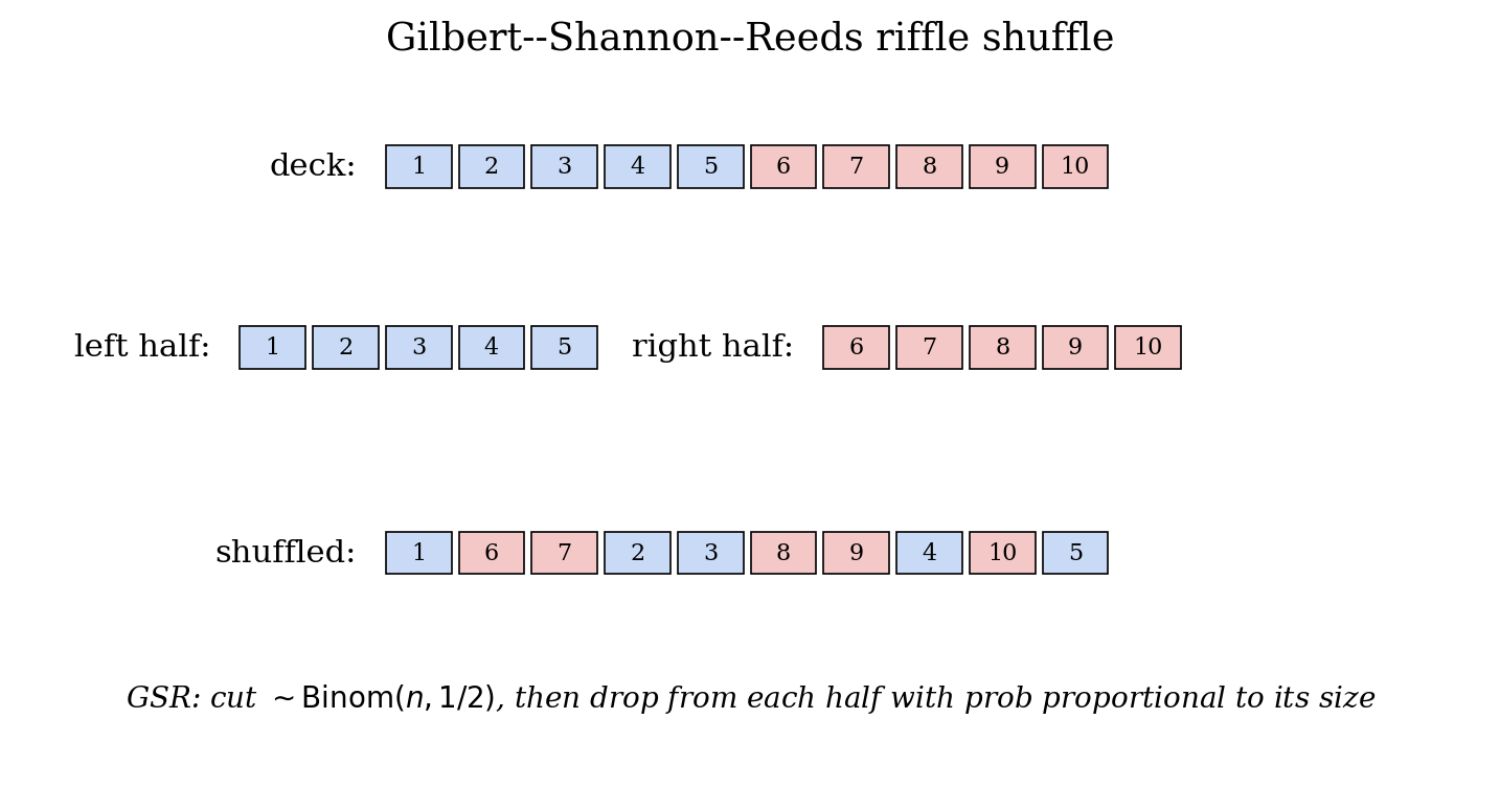
Example 5.4. The Gilbert–Shannon–Reeds model of card shuffling uses ergodic theory to analyze riffle shuffles.

5.3 Number Theory

We can also use ergodic theory to study number theory. The key definition that allows us to make this connection is as follows:

Definition 5.5. The upper density of a subset $S$ of the natural numbers $\mathbb{N}$ is defined as

This upper density behaves “almost” like a measure, and a number of the proofs given for the measure-theoretic dynamics can be repeated for analogs with the upper density. The dynamics are then mostly given by translations of the natural numbers by a fixed difference $d$, to study arithmetic progressions. This allowed Furstenberg to present an ergodic-theoretic proof of Szemerédi’s theorem:

Theorem 5.6 (Szemerédi’s Theorem). Every set of integers $A$ with positive upper density contains a $k$-term arithmetic progression for every $k$.

The ergodic-theoretic proof is given by effectively proving the Poincaré recurrence theorem for the “measure” given by an upper density, and for the dynamics given by $+d$, for some integer $d > 0$. Containing a $k$-term arithmetic progression is thus equivalent to the set having a $k$-recurrent subset.

Even though the prime numbers have $0$ upper density by the Prime Number Theorem, Green–Tao were able to extend these methods to show that the prime numbers contain arbitrarily long arithmetic progressions.

Theorem 5.7. Almost all invertible measure-preserving transformations are weak-mixing. More formally, for a given probability space $(X, \mathcal{X}, \mu)$, we can form the space $\mathrm{Aut}(X, \mu)$ of all measure-preserving transformations, and give it a weak topology. In this topology, the weak-mixing transformations form a dense $G_\delta$ set (a residual set).

The end of the last section also motivates a natural next area of study. Since spectral invariants are too weak to distinguish different systems with continuous spectrum from each other, we must find a stronger notion of invariance. Kolmogorov and Sinai did this by creating the notion of entropy of a dynamical system, which has become an active area of research. Entropy can be defined in both the topological and the measure-theoretic setting, and discussing it is beyond the scope of these notes. The motivated reader is referred to [2].

References

1. Eisner, T., Farkas, B., Haase, M., & Nagel, R. (2015). Operator-Theoretic Aspects of Ergodic Theory. Springer.
2. Walters, P. (1982). An Introduction to Ergodic Theory. Graduate Texts in Mathematics, Vol. 79. Springer-Verlag, New York. ISBN 0-387-90599-5.
3. Chacon, R. V. (1969). Weakly mixing transformations which are not strongly mixing. Proceedings of the American Mathematical Society, 22, 559–562.